
A Practical Oval Allocation Case Study
How to Simultaneously Achieve Higher Yield and Better Optical Performance for Oval Cuts
-
Thursday, 30 July 2026, 2:00 PM – 5:00 PM
-
Sunil Panchal +91-9879589682
-
Registration Closed
add event to your calendar
In our previous presentations, "Parameter-Based Allocation vs. 3D Node Model-Based Allocation" (May 6, 2025) and "Dead Zones vs. Dynamical Contrast: Where Is the Boundary of High-Performance Cuts?", we demonstrated the advantages of 3D Node Model-Based Allocation over traditional parameter-based approaches and showed how to distinguish diamonds affected by Dead Zones from those exhibiting High Dynamical Contrast.
This new presentation focuses on the practical application of these concepts by combining 3D Node Model-Based Allocation with Dead Zone analysis in a real production scenario.
Traditional planning is based on Main Parameters, which are typically defined by the Range Limits and include 5 key parameters: Girdle Ratio, Table Size, Crown Angle, Pavilion Angle, and Girdle Thickness.
The remaining geometric variables are referred to as Additional Parameters and are not considered in the traditional planning approach. In this study, we vary 7 Additional Parameters: Pavilion Main Curve Azimuth, Pavilion Main Point Azimuth, Pavilion Halves Curve, Wing, and Point Slopes, and Crown Main Wing and Point Slopes. The complete set of Additional Parameters is considerably larger.
This new presentation focuses on the practical application of these concepts by combining 3D Node Model-Based Allocation with Dead Zone analysis in a real production scenario.
Traditional planning is based on Main Parameters, which are typically defined by the Range Limits and include 5 key parameters: Girdle Ratio, Table Size, Crown Angle, Pavilion Angle, and Girdle Thickness.
The remaining geometric variables are referred to as Additional Parameters and are not considered in the traditional planning approach. In this study, we vary 7 Additional Parameters: Pavilion Main Curve Azimuth, Pavilion Main Point Azimuth, Pavilion Halves Curve, Wing, and Point Slopes, and Crown Main Wing and Point Slopes. The complete set of Additional Parameters is considerably larger.
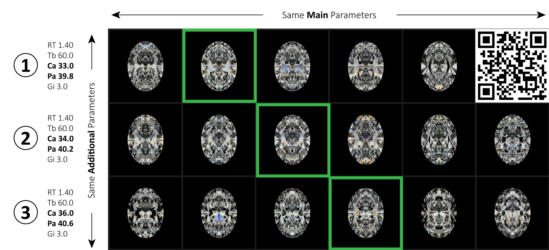
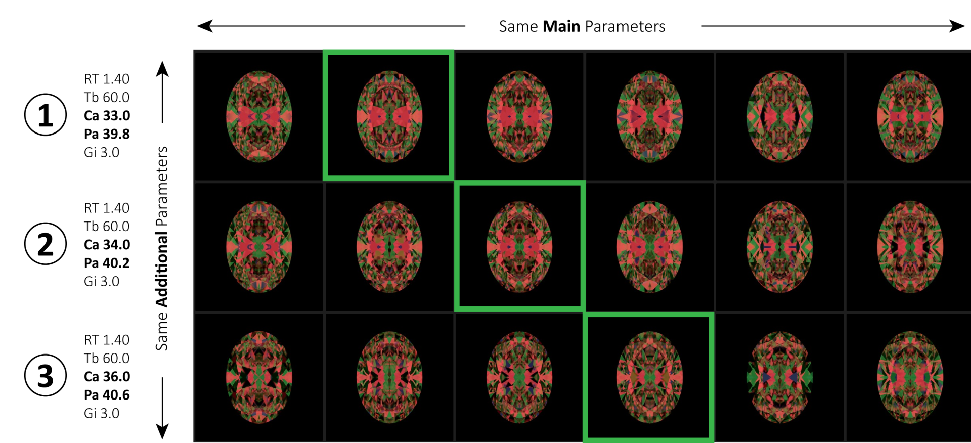
To illustrate their influence, we selected three different combinations of the 5 Main Parameters:
-
RT 1.40, Tb 60, Ca 33, Pa 39.8, Gi 3
-
RT 1.40, Tb 60, Ca 34, Pa 40.2, Gi 3
-
RT 1.40, Tb 60, Ca 36, Pa 40.6, Gi 3
In the figure (https://cutwise.com/~l6UF), each row represents one fixed combination of Main Parameters, while each column represents one fixed combination of Additional Parameters.
Despite having identical Main Parameters, the ovals within the same row exhibit noticeably different Optical Performance. This demonstrates that Additional Parameters can either enhance or degrade the optical performance of a given Main Parameter combination.
The best-performing oval in each row is highlighted in green. Notice that the optimal Additional Parameters are different for each set of Main Parameters.
This leads to two important conclusions:
Despite having identical Main Parameters, the ovals within the same row exhibit noticeably different Optical Performance. This demonstrates that Additional Parameters can either enhance or degrade the optical performance of a given Main Parameter combination.
The best-performing oval in each row is highlighted in green. Notice that the optimal Additional Parameters are different for each set of Main Parameters.
This leads to two important conclusions:
-
There is no universal set of Additional Parameters that produces high Optical Performance for every combination of Main Parameters.
-
Likewise, there is no "Ideal" set of Main Parameters that guarantees high optical performance regardless of the Additional Parameters.
High optical performance is achieved only through the proper combination of both Main and Additional Parameters.
Traditional planning is based only on the Main Parameters. As a result, the planner can optimize the target weight by selecting proportions within the Range Limits, but cannot directly control the final Optical Performance. Instead, the Optical Performance is determined later by the polisher through the choice of Additional Parameters.
3D Node Model-Based Allocation removes this limitation by optimizing both Main and Additional Parameters simultaneously. This enables the selection of allocation solutions that achieve both higher Yield and improved Optical Performance, including higher Brilliance and reduced Dead Zones.
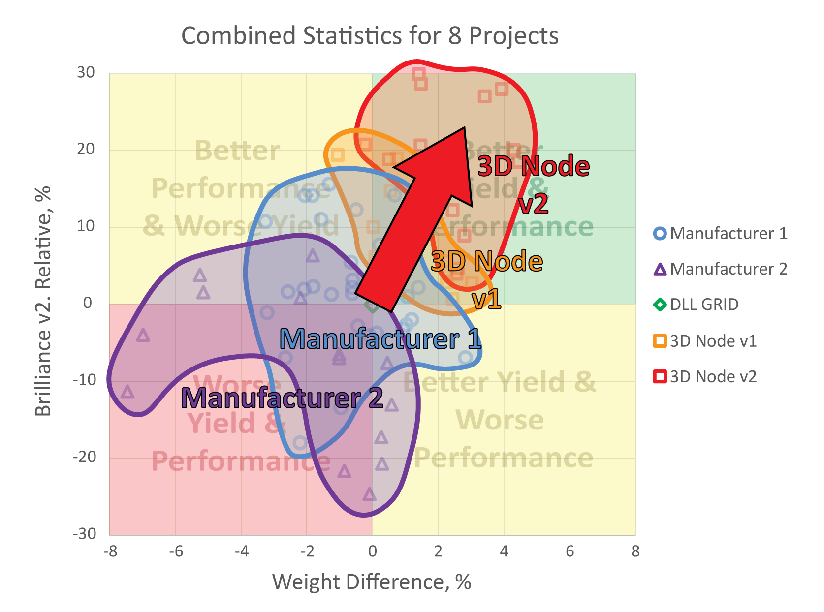
The figure below summarizes the results for 8 makeable projects. The DLL GRID solution is used as the reference, and all other solutions are plotted as the relative differences in Yield (horizontal axis) and Brilliance v2 (vertical axis). The comparison includes typical manufacturing solutions, 3D Node v1, and 3D Node v2 solutions.
Solutions located in the upper-right quadrant simultaneously achieve higher Yield and higher Brilliance than the reference solution. In contrast, solutions in the lower-left quadrant perform worse than the reference in both metrics.
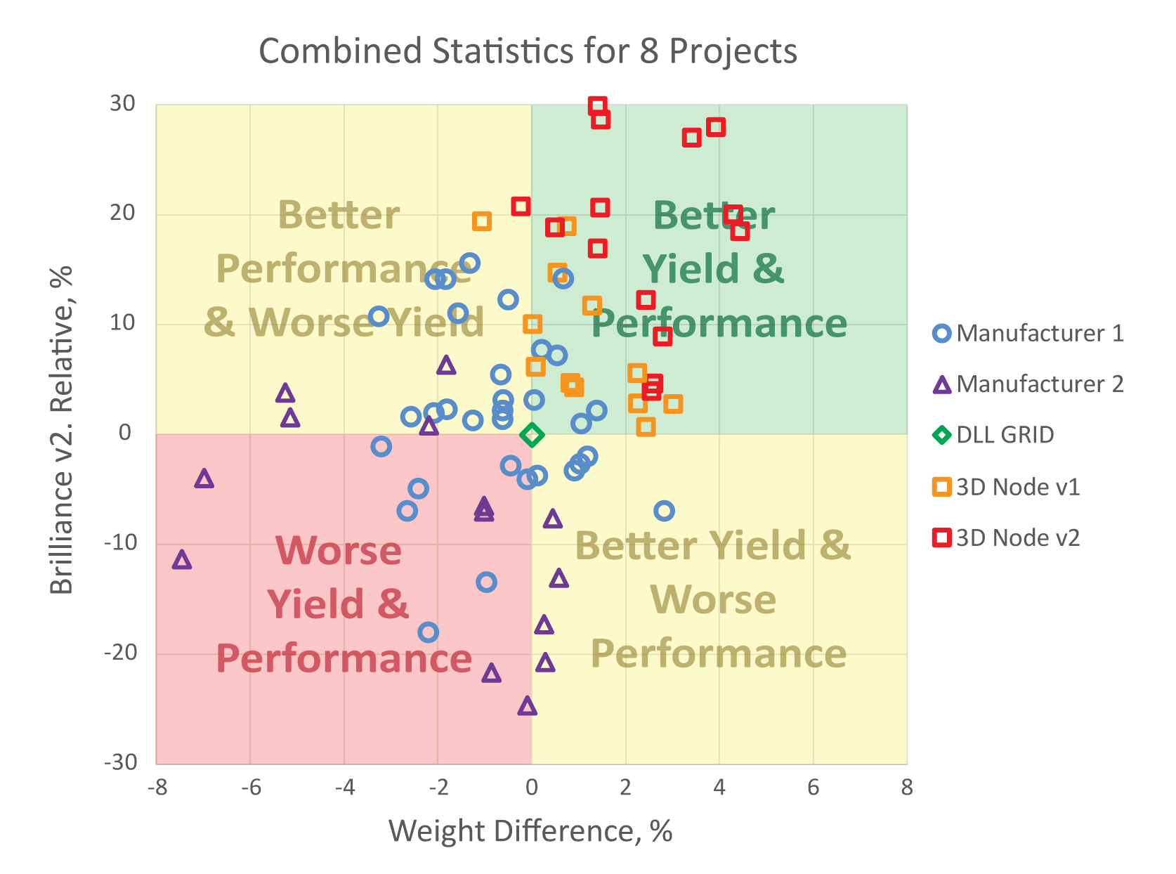
The distribution of the points clearly shows that different appraisers occupy different regions of the diagram. This reflects the quality of the preform libraries used by each planning method.
As a result, companies that systematically develop and refine their own 3D preform libraries will gain a significant competitive advantage. Even when using the same planning software and the same ranges of Main Parameters, they will be able to achieve higher Yield and better Optical Performance than companies that rely on a static or poorly optimized preform library.
Updating the preform library from 3D Node v1 to 3D Node v2 shifts the solutions toward the upper-right quadrant, demonstrating simultaneous improvements in both Yield and Brilliance.
Unlike traditional planning systems that rely on a fixed set of preforms, the 3D Node preform library is continuously expandable. Every newly discovered high-performing combination of Main and Additional Parameters can be added to the library, enabling planning quality to improve continuously over time.
As a result, companies that systematically develop and refine their own 3D preform libraries will gain a significant competitive advantage. Even when using the same planning software and the same ranges of Main Parameters, they will be able to achieve higher Yield and better Optical Performance than companies that rely on a static or poorly optimized preform library.
To make the session as practical as possible, we recommend that all participants download the provided set of makeable rough models and the reference Oval Range Limits before the presentation. We encourage you to generate allocation plans both within these reference Range Limits and within the Range Limits currently used at your own factory.
During the practical session after the presentation, you will be able to compare your own solutions with those generated using our new 3D Node appraisers. This direct comparison will help you better understand the potential of the technology and evaluate the practical benefits it could bring to your production.
New Challenge
We are also launching an Allocation Challenge based on these projects. Submit your best allocation solutions for the provided rough models, and the best-performing entries will receive prizes.
The competition rules, evaluation criteria, and submission instructions will be published at the following link:
© 2026 Octonus Finland Oy
All rights reserved
All rights reserved
Social
Created with